ESS 330 Final Project: Changes in Carbon Emissions and Energy Use in the Top Five Polluting Countries During COVID-19

Introduction/Hypothesis

Climate change is one of the most urgent challenges facing the world today. A primary driver of climate change is the release of greenhouse gases, especially carbon dioxide (CO₂), which is emitted through activities such as burning fossil fuels for energy, transportation, and industrial processes. CO₂ remains the most significant contributor to global warming due to its long atmospheric lifespan and the scale of human emissions Archer et al. (2009). Despite international agreements like the Paris Accord aimed at limiting global warming, CO₂ emissions continue to rise Programme (2022).

A small number of countries—China, the United States, India, Russia, and Japan—are responsible for the majority of global carbon emissions. These nations differ in population size, energy sources, and industrial output, yet each plays a critical role in shaping emissions trends. Assessing emissions on a per capita basis provides a more equitable way to understand responsibility and consumption, offering deeper insights than total emissions alone (Ritchie202?).

The COVID-19 pandemic created an unexpected opportunity to examine how major disruptions impact emissions. In 2020, global CO₂ emissions fell by approximately 5.4 percent, the largest annual drop ever recorded (Forster et al., 2020), largely due to reduced transportation and industrial activity during lockdowns. However, as economies reopened in 2021 and 2022, emissions quickly rebounded. This raises important questions about whether these changes signal structural shifts or were merely temporary (lequere2021?).

Energy-related emissions are a critical factor in understanding changes in CO₂ output, especially as global energy demand continues to grow. Each country’s energy mix—how it generates electricity—affects the amount of CO₂ emitted per kilowatt-hour. This makes energy-based metrics essential for comparing emissions and identifying opportunities for reductions.

While some studies have examined the short-term impacts of COVID-19 on emissions, fewer have investigated long-term trends in per capita and energy-related emissions across the highest-emitting countries. This study addresses that gap by applying both traditional statistical analysis and machine learning techniques to explore emission trends from 2015 to 2022 in China, the United States, India, Russia, and Japan.

We focus on two main indicators: greenhouse gas emissions per person and CO₂ emissions per kilowatt-hour of energy used. Data are divided into three periods: pre-COVID (2015–2019), during COVID (2020), and post-COVID (2021–2022). By comparing these periods, we aim to determine whether emission shifts were lasting or temporary and to identify the sectors that contributed most to these changes.

Objectives 

1. Compare per capita greenhouse gas emissions before, during, and after COVID-19 in the five largest CO₂-emitting countries. 

2. Identify which sector-specific emissions best predict per capita and per unit energy CO₂ emissions using linear regression and machine learning. 

3. Evaluate whether emission changes during the pandemic represent meaningful shifts in national emissions behavior. 

Hypotheses 

• H1: Per capita greenhouse gas emissions declined during the COVID-19 pandemic and partially rebounded in the post-COVID period, with variation across countries. 

• H2: Sector-specific emissions such as gas and coal use are strong predictors of per capita emissions in all periods. 

• H3: GDP per capita and gas emissions per capita are the most important predictors of CO₂ emissions per unit of energy. 

Methods

Study Scope and Dataset

Greenhouse gas emissions data was sourced from Our World in Data (Samborska, 2025), which compiles information from multiple sources, such as the Global Carbon Project. The dataset from Oxford’s Our World in Data includes emissions levels from the industrial revolution up to 2023. We utilized data from 2015 to 2022, focusing on the years 2019 to 2021, with the peak of the COVID-19 pandemic lockdowns happening in 2020 (forster2020current?).

To explain influences on total CO2, we narrowed 78 metrics collected in the Oxford dataset to two response variables, CO2 per unit energy, and CO2 emissions per capita (excluding land use change). These response variables account for regular widespread emissions. The proportion of per capita emissions from the top five cumulative CO2 emitting countries to the full record of countries during the 2015 to 2022 period revealed the impact that these countries can have to curb CO2 emissions in the future. In 2022, the top five CO2 emitters were responsible for 60.9 percent of global CO2 emissions.

Data Preparation and Predictor Variables

To compare CO2 emissions before, during, and after the pandemic, we used the tidymodels package in R along with dplyr. The predictor variables gdp_percap, gas_CO2_per_capita, share_global_coal_CO2, coal_CO2_per_capita, cumulative_luc_CO2, oil_CO2_per_capita, and share_global_luc_CO2 (Table 1) were chosen to model CO2 emissions per unit energy based on correlation tests and an educated guess as to the most effective predictors. These predictor variables attributed the response partly to individual demand for energy (in the case of per capita emissions) and partly to energy use by the whole country (in the case of share of global coal CO2 emissions). Although there are many energy sources for electricity, coal is the most CO2-polluting, so was one of the only two energy polluters included E. P. Agency (2025).

Predictor variables for ghg_excluding_lucf_per_capita were cumulative_CO2_including_luc, primary_energy_consumption, temperature_change_from_ghg, population, CO2_per_unit_energy, gdp_percap, cumulative_CO2, cumulative_coal_CO2, cumulative_coal_CO2, cumulative_luc_CO2, energy_per_capita. These predictors attempted to find a proxy for population-based CO2 emissions.

Statistical and Machine Learning Methods

To analyze our data, we used a combination of ANOVA statistical tests and machine learning. ANOVA was used to assess differences in emissions before, during, and after COVID. A linear regression model was used to model per-capita emissions as a function of sector-specific CO2 emissions (coal, oil, gas, cement, and misc industry). Our research focuses on revealing relationships between countries and between predictor variables of greenhouse emissions.

We compared per unit energy CO2 emissions among the top five cumulative polluters. Machine learning models to predict ghg_excluding_lucf_per_capita (greenhouse gases excluding land use change emitted per person) and CO2_per_unit_energy (in CO2 emitted per kilowatt-hour) were constructed using the rsamples, parsnip, workflowsets, and baguettes packages.

We tested predictor variables with linear regression, neural network Giannelos et al. (2024), random forest (Kjajavi et al. 2023), decision tree Rahman et al. (2023), and boosted tree Si & Du (2020) models to find predictor variables. The best model for each of the two response variables was analyzed with the vip package to reveal the most explanatory variables that predicted CO2 emissions per unit energy and CO2 per capita emissions from the selected variables.

Results

Data Exploration

In [1]:

library(tidyverse)

── Attaching core tidyverse packages ──────────────────────── tidyverse 2.0.0 ──
✔ dplyr     1.1.4     ✔ readr     2.1.5
✔ forcats   1.0.0     ✔ stringr   1.5.1
✔ ggplot2   3.5.2     ✔ tibble    3.2.1
✔ lubridate 1.9.4     ✔ tidyr     1.3.1
✔ purrr     1.0.4     
── Conflicts ────────────────────────────────────────── tidyverse_conflicts() ──
✖ dplyr::filter() masks stats::filter()
✖ dplyr::lag()    masks stats::lag()
ℹ Use the conflicted package (<http://conflicted.r-lib.org/>) to force all conflicts to become errors

library(readr)
library(ggplot2)
library(tidyr)
library(dplyr)

data <- read_csv("data/owid-co2-data (1).csv")

Rows: 50191 Columns: 79
── Column specification ────────────────────────────────────────────────────────
Delimiter: ","
chr  (2): country, iso_code
dbl (77): year, population, gdp, cement_co2, cement_co2_per_capita, co2, co2...

ℹ Use `spec()` to retrieve the full column specification for this data.
ℹ Specify the column types or set `show_col_types = FALSE` to quiet this message.

In [2]:

# Narrowing Data to 2015-2022
data_filtered <- data |> 
  filter(year >= 2015, year <= 2022) |> 
  filter(!is.na(iso_code) & nchar(iso_code) == 3)

# Getting top 5 CO2 emitting countries by total GHG (excluding land use)- This is total cumulative ghg emissions
top_emitters <- data_filtered |> 
  group_by(country) |> 
  summarise(total_ghg = sum(total_ghg_excluding_lucf, na.rm = TRUE)) |> 
  arrange(desc(total_ghg)) |> 
  slice_head(n = 5) |> 
  pull(country)

# Filtering data to include only those countries and select relevant variables
df <- data_filtered |> 
  filter(country %in% top_emitters) |> 
  select(country, year, ghg_excluding_lucf_per_capita, 
         coal_co2, gas_co2, oil_co2, cement_co2, other_industry_co2)

# Adding period category (pre, during, post COVID)
df <- df |> 
  mutate(period = case_when( 
    year <= 2019 ~ "pre_covid", 
    year == 2020 ~ "during_covid", 
    year >= 2021 ~ "post_covid" 
  )) |> 
  mutate(period = factor(period, levels = c("pre_covid", "during_covid", "post_covid")))

In [3]:

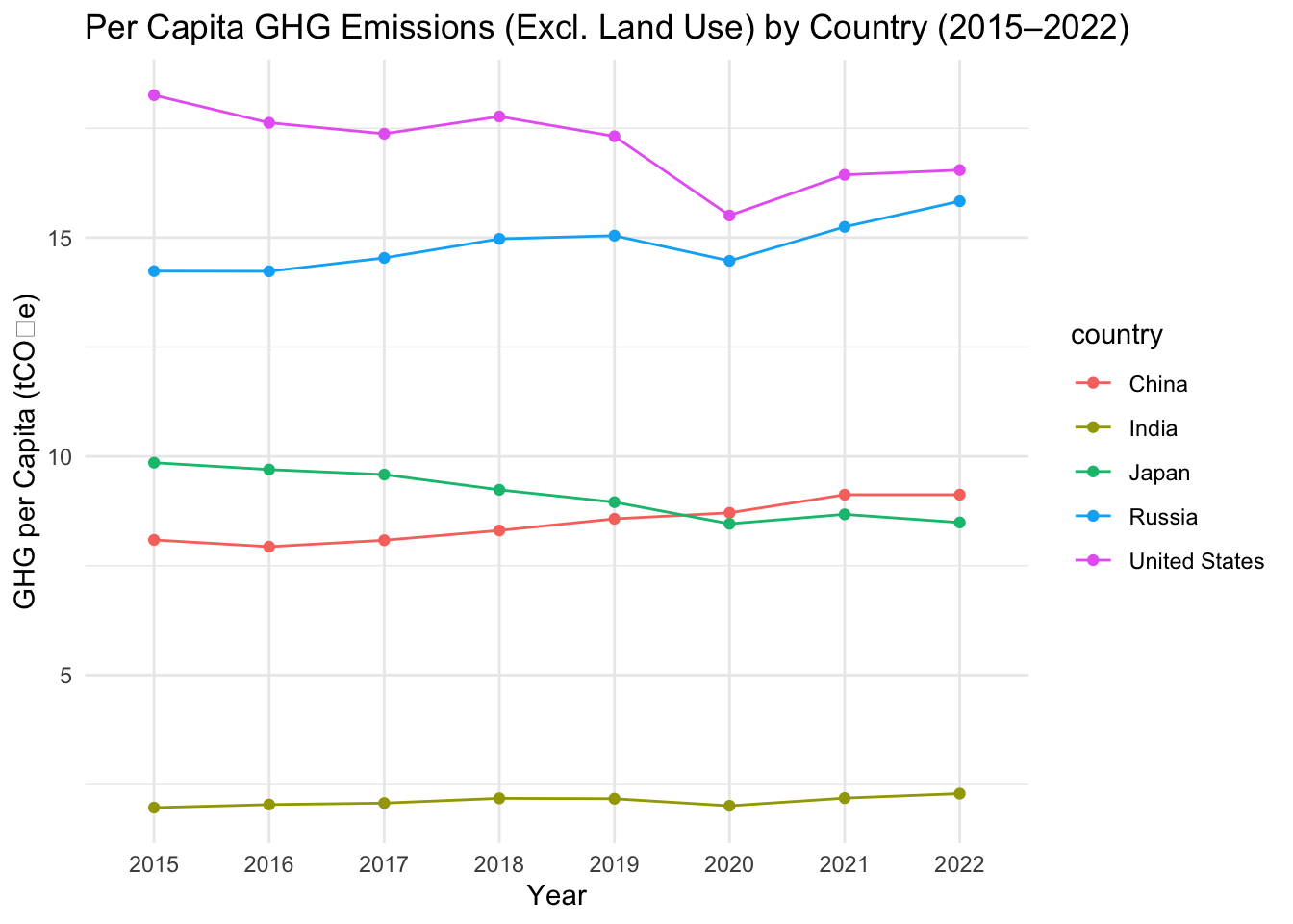
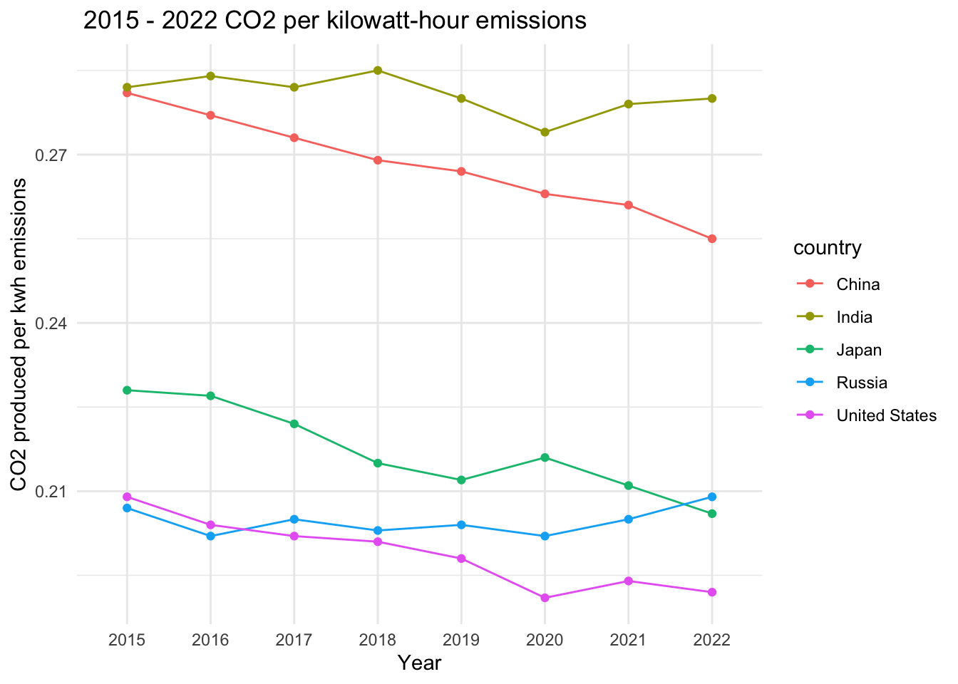
knitr::opts_chunk$set(
  echo = FALSE,       
  warning = FALSE,    
  message = FALSE)    
ggplot(df, aes(x = factor(year), y = ghg_excluding_lucf_per_capita, color = country, group = country)) +
  geom_line() +
  geom_point() +
  labs(
    title = "Per Capita GHG Emissions (Excl. Land Use) by Country (2015–2022)",
    x = "Year", y = "GHG per Capita (tCO₂e)"
  ) +
  theme_minimal()

Figure 1: This graph shows how greenhouse gas emissions per person changed in China, the United States, India, Russia, and Japan from 2015 to 2022. You can see a drop around 2020 during COVID, especially in the United States and Russia. Some countries’ emissions started going back up after 2020.

In [4]:

df_long <- df |> 
  pivot_longer(cols = c(coal_co2, gas_co2, oil_co2, cement_co2, other_industry_co2),
               names_to = "sector", values_to = "emissions") |> 
  drop_na(emissions)

ggplot(df_long, aes(x = year, y = emissions, color = sector, group = interaction(sector, country))) +
  geom_line() +
  geom_point() +
  facet_wrap(~ country, scales = "free_y", ncol = 2) +
  scale_x_continuous(breaks = 2015:2022) +
  labs(title = "Sector-specific CO₂ Emissions (2015–2022)", 
       x = "Year", 
       y = "Emissions (MtCO₂)") +
  theme_minimal() +
  theme(axis.text.x = element_text(angle = 45, hjust = 1))

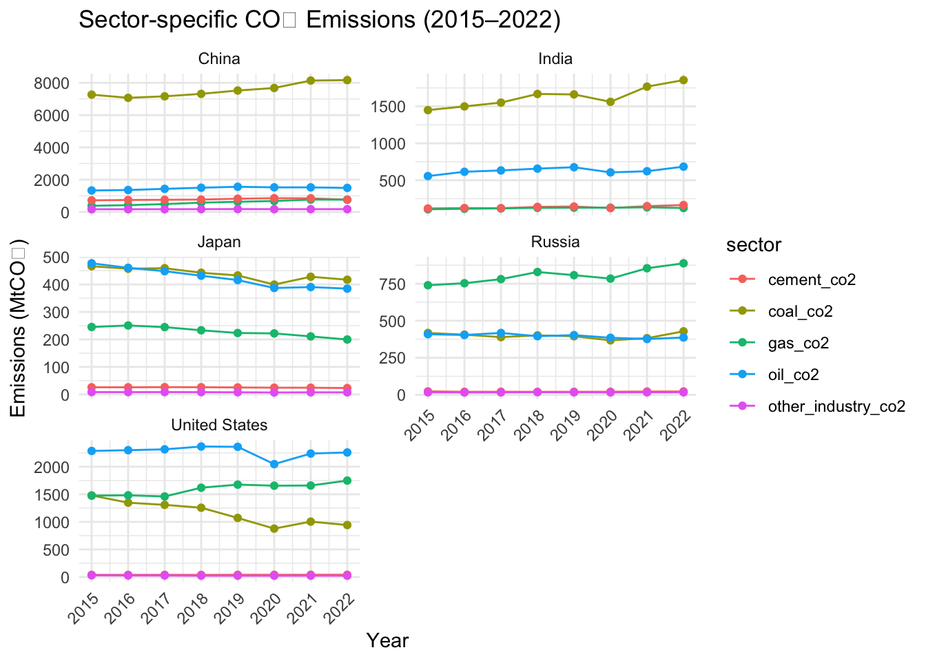
Figure 2: This graph shows where each country’s emissions came from: like coal, oil, gas, cement, or other industries. For example, China has a lot of coal emissions, and the United States has more oil emissions. You can also see how emissions from some sectors dropped in 2020 and then changed again after COVID.

In [5]:

knitr::opts_chunk$set(
  echo = FALSE,       
  warning = FALSE,    
  message = FALSE)    
# 1. Prepare data
df <- data_filtered |>
  filter(country %in% top_emitters) |>
  select(country, year, ghg_excluding_lucf_per_capita,
         coal_co2, gas_co2, oil_co2, cement_co2, other_industry_co2,
         gdp, population) |>
  mutate(
    gdp_per_capita = gdp / population,
    period = case_when(
      year <= 2019 ~ "pre_covid",
      year == 2020 ~ "during_covid",
      year >= 2021 ~ "post_covid"
    )
  ) |>
  mutate(period = factor(period, levels = c("pre_covid", "during_covid", "post_covid")))

# 2. Run ANOVA for each country
for (c in unique(df$country)) {
  df_country <- df |> filter(country == c)
  if (n_distinct(df_country$period) > 1) {
    cat("\n--- ANOVA for", c, "---\n")
    model <- aov(ghg_excluding_lucf_per_capita ~ period, data = df_country)
    print(summary(model))
  } else {
    cat("\n--- Skipped ANOVA for", c, ": not enough periods ---\n")
  }
}

--- ANOVA for China ---
            Df Sum Sq Mean Sq F value Pr(>F)  
period       2 1.2803  0.6402   13.06 0.0103 *
Residuals    5 0.2451  0.0490                 
---
Signif. codes:  0 '***' 0.001 '**' 0.01 '*' 0.05 '.' 0.1 ' ' 1

--- ANOVA for India ---
            Df  Sum Sq  Mean Sq F value Pr(>F)
period       2 0.04456 0.022280   2.956  0.142
Residuals    5 0.03769 0.007537               

--- ANOVA for Japan ---
            Df Sum Sq Mean Sq F value Pr(>F)  
period       2 1.6155  0.8077   7.299 0.0329 *
Residuals    5 0.5533  0.1107                 
---
Signif. codes:  0 '***' 0.001 '**' 0.01 '*' 0.05 '.' 0.1 ' ' 1

--- ANOVA for Russia ---
            Df Sum Sq Mean Sq F value Pr(>F)  
period       2 1.3923  0.6961   4.433 0.0781 .
Residuals    5 0.7852  0.1570                 
---
Signif. codes:  0 '***' 0.001 '**' 0.01 '*' 0.05 '.' 0.1 ' ' 1

--- ANOVA for United States ---
            Df Sum Sq Mean Sq F value  Pr(>F)   
period       2  4.906  2.4529   21.37 0.00355 **
Residuals    5  0.574  0.1148                   
---
Signif. codes:  0 '***' 0.001 '**' 0.01 '*' 0.05 '.' 0.1 ' ' 1

# 3. Linear Regression
lm_model <- lm(ghg_excluding_lucf_per_capita ~ coal_co2 + oil_co2 + gas_co2 + cement_co2 + other_industry_co2, data = df)
summary(lm_model)

Call:
lm(formula = ghg_excluding_lucf_per_capita ~ coal_co2 + oil_co2 + 
    gas_co2 + cement_co2 + other_industry_co2, data = df)

Residuals:
    Min      1Q  Median      3Q     Max 
-2.2833 -0.3541  0.1507  0.4693  1.4989 

Coefficients:
                     Estimate Std. Error t value Pr(>|t|)    
(Intercept)         8.2798981  0.3661956  22.611  < 2e-16 ***
coal_co2            0.0003590  0.0008477   0.424 0.675372    
oil_co2            -0.0021149  0.0005530  -3.825 0.000737 ***
gas_co2             0.0074705  0.0008038   9.293 9.53e-10 ***
cement_co2         -0.0237091  0.0076398  -3.103 0.004572 ** 
other_industry_co2  0.0864354  0.0379252   2.279 0.031111 *  
---
Signif. codes:  0 '***' 0.001 '**' 0.01 '*' 0.05 '.' 0.1 ' ' 1

Residual standard error: 0.9042 on 26 degrees of freedom
  (8 observations deleted due to missingness)
Multiple R-squared:  0.9521,    Adjusted R-squared:  0.9429 
F-statistic: 103.3 on 5 and 26 DF,  p-value: 2.663e-16

Country	p-value	Interpretation
China	0.0103	Significant change (p < 0.05)
India	0.142	No significant change (p > 0.05)
Japan	0.0329	Significant change (p < 0.05)
Russia	0.0781	Not quite significant (p > 0.05)
United States	0.00355	Significant change (p < 0.01)

In [6]:

#Rebuilding top emitters and running ANOVA
top_emitters <- data_filtered |>
  filter(year >= 2015, year <= 2022) |>
  group_by(country) |>
  summarise(total_ghg = sum(total_ghg_excluding_lucf, na.rm = TRUE)) |>
  slice_max(total_ghg, n = 5) |>
  pull(country)

df <- data_filtered |>
  filter(country %in% top_emitters, year >= 2015, year <= 2022) |>
  mutate(
    ghg_per_eny = co2_per_unit_energy,
    period = case_when(
      year <= 2019 ~ "pre_covid",
      year == 2020 ~ "during_covid",
      year >= 2021 ~ "post_covid"
    ),
    period = factor(period, levels = c("pre_covid", "during_covid", "post_covid"))
  )

anova_results <- tibble(
  country = character(),
  p_value = numeric()
)


for (c in unique(df$country)) {
  df_country <- df |> filter(country == c)
  if (n_distinct(df_country$period) > 1) {
    model <- aov(ghg_per_eny ~ period, data = df_country)
    p_val <- summary(model)[[1]][["Pr(>F)"]][1]

    anova_results <- anova_results |> add_row(
      country = c,
      p_value = p_val
    )
  }
}

#p value interpret
anova_results <- anova_results |>
  mutate(
    p_value = signif(p_value, 5),
    Interpretation = case_when(
      p_value < 0.01 ~ "Significant change (p < 0.01)",
      p_value < 0.05 ~ "Significant change (p < 0.05)",
      p_value < 0.10 ~ "Not quite significant (p > 0.05)",
      TRUE ~ "No significant change (p > 0.05)"
    )
  )

#table
cat("| Country         | p-value | Interpretation                         |\n")

| Country         | p-value | Interpretation                         |

cat("|-----------------|---------|-----------------------------------------|\n")

|-----------------|---------|-----------------------------------------|

for (i in 1:nrow(anova_results)) {
  row <- anova_results[i, ]
  cat(sprintf(
    "| %-15s | %-7.5f | %-39s |\n",
    row$country,
    row$p_value,
    row$Interpretation
  ))
}

| China           | 0.04420 | Significant change (p < 0.05)           |
| India           | 0.01629 | Significant change (p < 0.05)           |
| Japan           | 0.17446 | No significant change (p > 0.05)        |
| Russia          | 0.21875 | No significant change (p > 0.05)        |
| United States   | 0.03078 | Significant change (p < 0.05)           |

In [7]:

lm_model <- lm(ghg_excluding_lucf_per_capita ~ coal_co2 + oil_co2 + gas_co2 + cement_co2 + other_industry_co2, data = df)
summary(lm_model)

Call:
lm(formula = ghg_excluding_lucf_per_capita ~ coal_co2 + oil_co2 + 
    gas_co2 + cement_co2 + other_industry_co2, data = df)

Residuals:
    Min      1Q  Median      3Q     Max 
-2.2833 -0.3541  0.1507  0.4693  1.4989 

Coefficients:
                     Estimate Std. Error t value Pr(>|t|)    
(Intercept)         8.2798981  0.3661956  22.611  < 2e-16 ***
coal_co2            0.0003590  0.0008477   0.424 0.675372    
oil_co2            -0.0021149  0.0005530  -3.825 0.000737 ***
gas_co2             0.0074705  0.0008038   9.293 9.53e-10 ***
cement_co2         -0.0237091  0.0076398  -3.103 0.004572 ** 
other_industry_co2  0.0864354  0.0379252   2.279 0.031111 *  
---
Signif. codes:  0 '***' 0.001 '**' 0.01 '*' 0.05 '.' 0.1 ' ' 1

Residual standard error: 0.9042 on 26 degrees of freedom
  (8 observations deleted due to missingness)
Multiple R-squared:  0.9521,    Adjusted R-squared:  0.9429 
F-statistic: 103.3 on 5 and 26 DF,  p-value: 2.663e-16

In [8]:

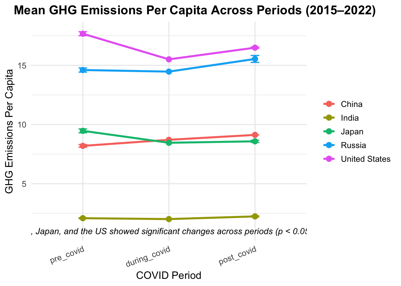
library(dplyr)
library(ggplot2)

# Example summary dataframe (replace with your actual grouped summary if needed)
summary_df <- df %>%
  group_by(country, period) %>%
  summarize(
    mean_emission = mean(ghg_excluding_lucf_per_capita, na.rm = TRUE),
    se = sd(ghg_excluding_lucf_per_capita, na.rm = TRUE) / sqrt(n()),
    .groups = "drop"
  )

# Optional: Set factor order for periods
summary_df$period <- factor(summary_df$period, levels = c("pre_covid", "during_covid", "post_covid"))

# Plot
ggplot(summary_df, aes(x = period, y = mean_emission, group = country, color = country)) +
  geom_line(linewidth = 1.2) +
  geom_point(size = 3) +
  geom_errorbar(aes(ymin = mean_emission - se, ymax = mean_emission + se), width = 0.1, linewidth = 0.7) +
  labs(
    title = "Mean GHG Emissions Per Capita Across Periods (2015–2022)",
    x = "COVID Period",
    y = "GHG Emissions Per Capita"
  ) +
  theme_minimal(base_size = 13) +
  theme(
    plot.title = element_text(hjust = 0.2, face = "bold"),
    axis.text.x = element_text(angle = 20, hjust = 1),
    legend.title = element_blank()
  ) +
  annotate("text", x = 2, y = min(summary_df$mean_emission) - 1,
           label = "Only China, Japan, and the US showed significant changes across periods (p < 0.05, ANOVA).",
           size = 3.8, hjust = 0.5, fontface = "italic")

Model Validation

• Plotted actual vs. predicted emissions to assess model fit.

• Visualized regression coefficients with confidence intervals to interpret the influence of each emission sector.

In [9]:

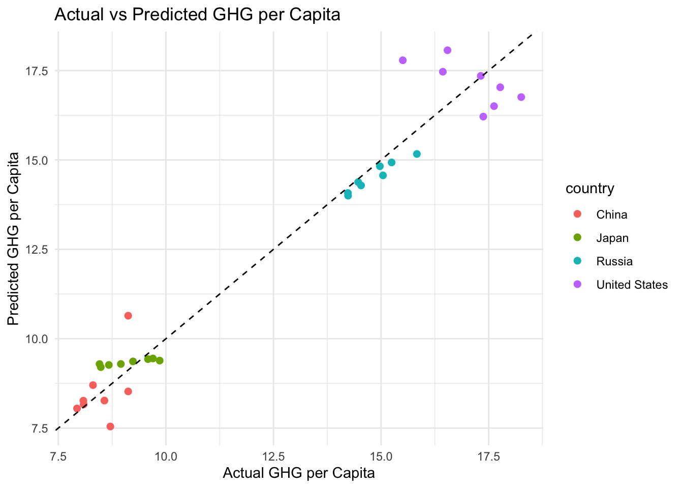
# After selecting the variables, clean properly:
df <- df |> drop_na(ghg_excluding_lucf_per_capita, coal_co2, oil_co2, gas_co2, cement_co2, other_industry_co2)

# Now build the model
lm_model <- lm(ghg_excluding_lucf_per_capita ~ coal_co2 + oil_co2 + gas_co2 + cement_co2 + other_industry_co2, data = df)

# Now add predictions
df$predicted <- predict(lm_model)

# Now plot Actual vs Predicted
ggplot(df, aes(x = ghg_excluding_lucf_per_capita, y = predicted, color = country)) +
  geom_point(size = 2) +
  geom_abline(slope = 1, intercept = 0, linetype = "dashed") +
  labs(title = "Actual vs Predicted GHG per Capita",
       x = "Actual GHG per Capita",
       y = "Predicted GHG per Capita") +
  theme_minimal()

Figure 3: This graph compares the real emissions to the ones predicted by our model. If the points are close to the dashed line, it means the model did a good job. Most of the points are pretty close to the line, so the model worked well.

Machine Learning Modeling

We conducted two separate modeling analyses to predict greenhouse gas (GHG) emissions per capita (excluding land use change) and CO2 emissions per kilowatt-hour, focusing on the top five global emitters between 2015 and 2022. Below we detail the results, supported by figures, tables, and the corresponding R code used for each step.

In [10]:

library(tidyverse)
library(readr)
library(ggplot2)
library(tidyr)
library(dplyr)


data <- read_csv("data/owid-co2-data (1).csv")

Rows: 50191 Columns: 79
── Column specification ────────────────────────────────────────────────────────
Delimiter: ","
chr  (2): country, iso_code
dbl (77): year, population, gdp, cement_co2, cement_co2_per_capita, co2, co2...

ℹ Use `spec()` to retrieve the full column specification for this data.
ℹ Specify the column types or set `show_col_types = FALSE` to quiet this message.

In [11]:

# Narrowing Data to 2015-2022

data_filtered <- data |>
  filter(year >= 2015, year <= 2022) |>
  filter(!is.na(iso_code) & nchar(iso_code) == 3)

In [12]:

# Getting top 5 CO2 emitting countries by total GHG (excluding land use)- This is total cumulative ghg emissions

top_emitters <- data_filtered |>
  group_by(country) |>
  summarise(total_ghg = sum(total_ghg_excluding_lucf, na.rm = TRUE)) |>
  arrange(desc(total_ghg)) |>
  slice_head(n = 5) |>
  pull(country)

# Filtering data to include only those countries and select relevant variables
df <- data_filtered |>
  filter(country %in% top_emitters) |>
  select(country, year, ghg_excluding_lucf_per_capita,
         coal_co2, gas_co2, oil_co2, cement_co2, other_industry_co2)

In [13]:

# Adding period category (pre, during, post COVID)
df <- df |>
  mutate(period = case_when(
    year <= 2019 ~ "pre_covid",
    year == 2020 ~ "during_covid",
    year >= 2021 ~ "post_covid"
  )) |>
  mutate(period = factor(period, levels = c("pre_covid", "during_covid", "post_covid")))

Table 1. A Table of Predictor Variables

In [14]:

# Load required libraries
library(gridExtra)

Attaching package: 'gridExtra'

The following object is masked from 'package:dplyr':

    combine

library(grid)
library(gtable)
library(png)

# Create a data frame with the model information
model_info <- data.frame(
  Model = c("Model 1", "Model 2"),
  Response_Variable = c("ghg_excluding_lucf_per_capita", "co2_per_unit_energy"),
  Predictors = c(
    "• cumulative_co2_including_luc\n• primary_energy_consumption\n• temperature_change_from_ghg\n• population\n• co2_per_unit_energy\n• gdp_percap\n• cumulative_co2\n• cumulative_coal_co2\n• cumulative_luc_co2\n• energy_per_capita",
    "• gas_co2_per_capita\n• oil_co2_per_capita\n• gdp_percap\n• coal_co2_per_capita\n• share_global_coal_co2\n• cumulative_luc_co2\n• share_global_luc_co2"
  )
)

# Create a more detailed table for display
detailed_table <- data.frame(
  " " = c("Model", "Response Variable", "Predictor Variables"),
  "Model 1" = c(
    "Model 1",
    "ghg_excluding_lucf_per_capita",
    paste(
      "• cumulative_co2_including_luc",
      "• primary_energy_consumption",
      "• temperature_change_from_ghg",
      "• population",
      "• co2_per_unit_energy",
      "• gdp_percap",
      "• cumulative_co2",
      "• cumulative_coal_co2",
      "• cumulative_luc_co2",
      "• energy_per_capita",
      sep = "\n"
    )
  ),
  "Model 2" = c(
    "Model 2",
    "co2_per_unit_energy",
    paste(
      "• gas_co2_per_capita",
      "• oil_co2_per_capita",
      "• gdp_percap",
      "• coal_co2_per_capita",
      "• share_global_coal_co2",
      "• cumulative_luc_co2",
      "• share_global_luc_co2",
      sep = "\n"
    )
  )
)

tg <- tableGrob(
  detailed_table, 
  rows = NULL,
  theme = ttheme_default(
    core = list(
      bg_params = list(fill = c("#F7F7F7", "#FFFFFF", "#F7F7F7"), col = NA),
      fg_params = list(cex = 0.8)
  )
))

# Add borders
tg <- gtable_add_grob(
  tg,
  grobs = rectGrob(gp = gpar(fill = NA, lwd = 2)),
  t = 1, b = nrow(tg), l = 1, r = ncol(tg)
)

# Add header background
tg <- gtable_add_grob(
  tg,
  grobs = rectGrob(gp = gpar(fill = "#4472C4", alpha = 0.5)),
  t = 1, l = 1, r = ncol(tg)
)

# Add white text for header
tg <- gtable_add_grob(
  tg,
  grobs = textGrob(
    "Predictor Variables for Machine Learning Models", 
    gp = gpar(fontface = "bold", col = "white", cex = 1.2)
  ),
  t = 1, l = 1, r = ncol(tg)
)

# Save as PNG
png("model_predictors_table.png", width = 800, height = 400, res = 100)
grid.draw(tg)
dev.off()

quartz_off_screen 
                2 

# Message to user
cat("Table saved as 'model_predictors_table.png' in your working directory:", getwd())

Table saved as 'model_predictors_table.png' in your working directory: /Users/amhs5/Documents/ESS330-FinalProject-April23

Predicting CO2 Emissions per capita

In [15]:

## Mutate data, check for Interaction terms

#set a seed
set.seed(341)

#doing a correlation test for variables

ghg_per_cap <- data_filtered %>% 
  mutate(period = case_when(
    year <= 2019 ~ "pre_covid",
    year == 2020 ~ "during_covid",
    year >= 2021 ~ "post_covid"
  )) %>% 
  group_by(country) %>% 
  mutate(gdp_percap = gdp/population) %>% 
  ungroup() %>% 
select(ghg_excluding_lucf_per_capita, cumulative_co2_including_luc, primary_energy_consumption, temperature_change_from_ghg, population, co2_per_unit_energy, gdp_percap, cumulative_co2, cumulative_coal_co2, cumulative_coal_co2, cumulative_luc_co2, energy_per_capita) %>%
  drop_na


pc_cor <- cor(ghg_per_cap)

#Interaction terms
#ghg_excluding_lucf_per_capita:energy_per_capita, gdp_percap:energy_per_capita, cumulative_luc_co2:cumulative_co2_including_luc, cumulative_luc_co2:temperature_change_from_n2o, cumulative_coal_co2:cumulative_co2, primary_energy_consumption:cumulative_coal_co2, temperature_change_from_ghg:cumulative_coal_co2, cumulative_coal_co2:temperature_change_from_n2o, temperature_change_from_co2:cumulative_coal_co2, cumulative_co2_including_luc:cumulative_coal_co2, temperature_change_from_ghg:cumulative_co2, primary_energy_consumption:cumulative_co2, ghg_excluding_lucf_per_capita:gdp_percap, primary_energy_consumption:population, cumulative_co2_including_luc:temperature_change_from_ghg, primary_energy_consumption:temperature_change_from_ghg, cumulative_luc_co2:temperature_change_from_ghg, primary_energy_consumption:cumulative_co2_including_luc, cumulative_co2:cumulative_co2_including_luc

In [16]:

#model workflow code

#find recipe format from lab 6 / model daily assignments
library(rsample)

ghg_per_cap_split <- initial_split(ghg_per_cap, prop = .8)
ghg_per_cap_train <- training(ghg_per_cap_split)
ghg_per_cap_test  <- testing(ghg_per_cap_split)


ghg_per_cap_cv <- vfold_cv(ghg_per_cap, v = 10)

In [17]:

#attempted recipe format
library(recipes)

Attaching package: 'recipes'

The following object is masked from 'package:stringr':

    fixed

The following object is masked from 'package:stats':

    step

rec_percap <- recipe(
  # Formula syntax: outcome ~ predictors
  ghg_excluding_lucf_per_capita ~ 
    cumulative_co2_including_luc + 
    primary_energy_consumption + 
    temperature_change_from_ghg + 
    population + 
    co2_per_unit_energy + 
    gdp_percap + 
    cumulative_co2 + 
    cumulative_coal_co2 + 
    cumulative_luc_co2 + 
    energy_per_capita, 
  data = ghg_per_cap
) %>%
  # Interaction terms (correct syntax)
  step_interact(
    terms = ~
      gdp_percap:energy_per_capita +
      cumulative_luc_co2:cumulative_co2_including_luc +
      cumulative_coal_co2:cumulative_co2 +
      primary_energy_consumption:cumulative_coal_co2 +
      temperature_change_from_ghg:cumulative_coal_co2 +
      cumulative_co2_including_luc:cumulative_coal_co2 +
      temperature_change_from_ghg:cumulative_co2 +
      primary_energy_consumption:cumulative_co2 +
      primary_energy_consumption:population +
      cumulative_co2_including_luc:temperature_change_from_ghg +
      primary_energy_consumption:temperature_change_from_ghg +
      cumulative_luc_co2:temperature_change_from_ghg +
      primary_energy_consumption:cumulative_co2_including_luc +
      cumulative_co2:cumulative_co2_including_luc
  ) %>% 
  step_naomit(all_predictors(), all_outcomes())

In [18]:

# Load required library
library(tidymodels)

── Attaching packages ────────────────────────────────────── tidymodels 1.3.0 ──

✔ broom        1.0.8     ✔ tune         1.3.0
✔ dials        1.4.0     ✔ workflows    1.2.0
✔ infer        1.0.8     ✔ workflowsets 1.1.0
✔ modeldata    1.4.0     ✔ yardstick    1.3.2
✔ parsnip      1.3.1     

── Conflicts ───────────────────────────────────────── tidymodels_conflicts() ──
✖ gridExtra::combine() masks dplyr::combine()
✖ scales::discard()    masks purrr::discard()
✖ dplyr::filter()      masks stats::filter()
✖ recipes::fixed()     masks stringr::fixed()
✖ dplyr::lag()         masks stats::lag()
✖ yardstick::spec()    masks readr::spec()
✖ recipes::step()      masks stats::step()

# Define your models
boost <- boost_tree(mode = "regression") %>%
  set_engine("xgboost")

nnet <- mlp(mode = "regression") %>%
  set_engine("nnet")

dtree <- decision_tree(mode = "regression") %>%
  set_engine("rpart")

rf <- rand_forest(mode = "regression") %>%
  set_engine("ranger", importance = "impurity")

In [19]:

## Plotting the best predictive models of emissions per unit energy

library(workflowsets)
library(baguette)

wfpc <-  workflow_set(list(rec_percap), 
                  list(boost,
                       nnet,
                       dtree,
                       rf)) %>%
  workflow_map('fit_resamples', resamples = ghg_per_cap_cv)

autoplot(wfpc) +
   theme(
    text = element_text(size = 10),
    axis.title = element_text(size = 12),
    axis.text = element_text(size = 8),
    plot.title = element_text(size = 14, face = "bold"),
    legend.title = element_text(size = 10),
    legend.text = element_text(size = 8)
  )

ggsave(
  filename = "imgs/percap_model_comparison.png",
  plot = last_plot(),
  width = 10,
  height = 6,
  dpi = 300
)

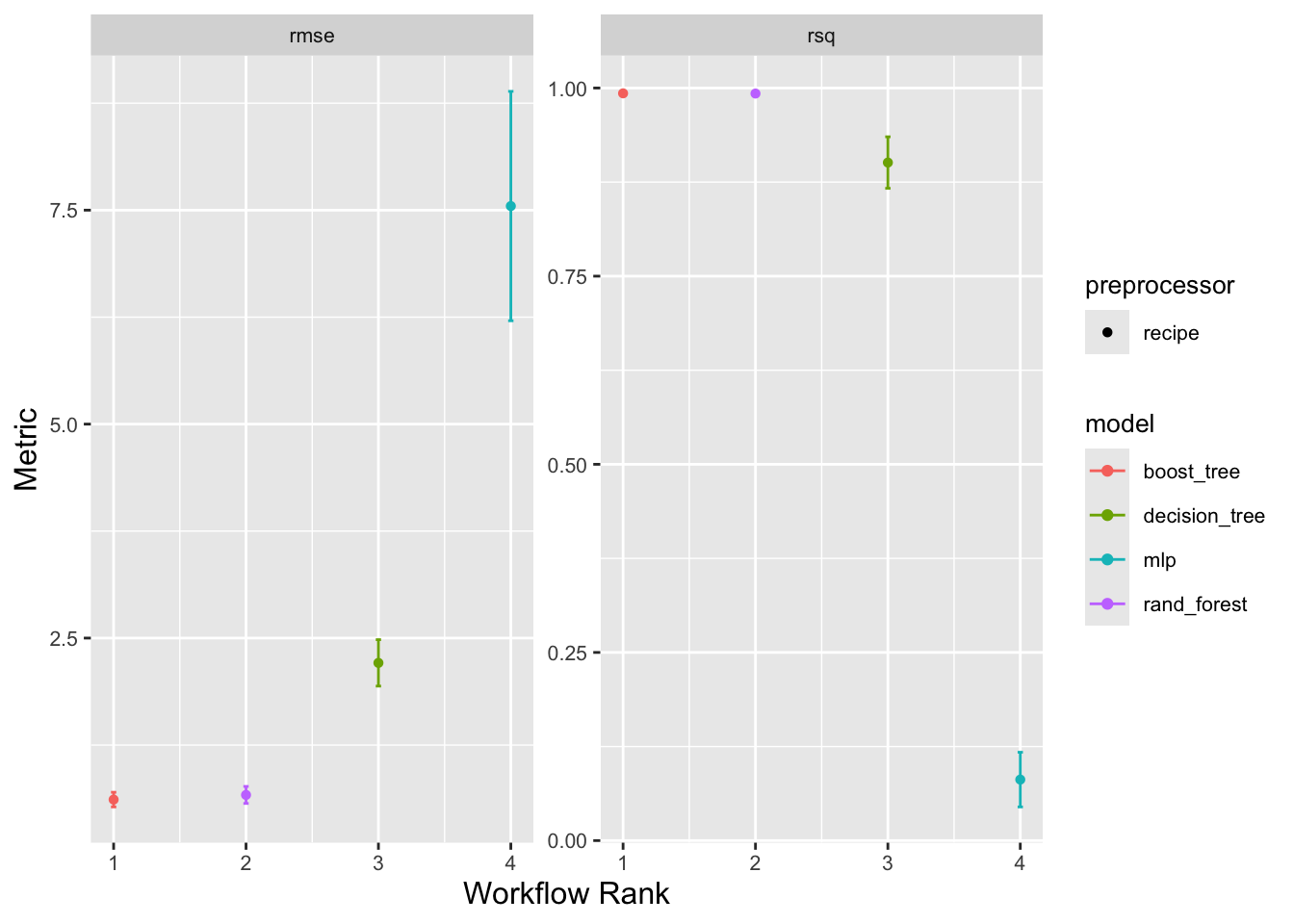
Figure 4. Ranking different models’ root mean squared error and R-squared error values, tested against CO2 per capita emissions data excluding land use change for the top five cumulative CO2 emitters.

Table 2. Ranking Model Testing Results

In [20]:

rank_results(wfpc, rank_metric = "rsq", select_best = TRUE)

# A tibble: 8 × 9
  wflow_id         .config .metric   mean std_err     n preprocessor model  rank
  <chr>            <chr>   <chr>    <dbl>   <dbl> <int> <chr>        <chr> <int>
1 recipe_boost_tr… Prepro… rmse    0.613  0.0521     10 recipe       boos…     1
2 recipe_boost_tr… Prepro… rsq     0.993  0.00161    10 recipe       boos…     1
3 recipe_rand_for… Prepro… rmse    0.667  0.0604     10 recipe       rand…     2
4 recipe_rand_for… Prepro… rsq     0.993  0.00149    10 recipe       rand…     2
5 recipe_decision… Prepro… rmse    2.21   0.165      10 recipe       deci…     3
6 recipe_decision… Prepro… rsq     0.901  0.0208     10 recipe       deci…     3
7 recipe_mlp       Prepro… rmse    7.55   0.815      10 recipe       mlp       4
8 recipe_mlp       Prepro… rsq     0.0811 0.0221     10 recipe       mlp       4

In [21]:

### Making a workflow to predict Co2 emitted per capita

library(tidymodels)
rf_wf_pc <- workflow() %>%
  # Add the recipe
  add_recipe(rec_percap) %>%
  # Add the model
  add_model(rf) %>%
  # Fit the model to the training data
  fit(data = ghg_per_cap_train) 

rf_data_pc <- augment(rf_wf_pc, new_data = ghg_per_cap_test)


dim(rf_data_pc)

[1] 192  12

In [22]:

## Ranking the most important predictors

rf_model <- extract_fit_engine(rf_wf_pc)
vip::vip(rf_model) + theme(
    text = element_text(size = 10),
    axis.title = element_text(size = 12),
    axis.text = element_text(size = 8),
    plot.title = element_text(size = 14, face = "bold"),
    legend.title = element_text(size = 10),
    legend.text = element_text(size = 8))

ggsave(filename = "compare_percap.png", plot = last_plot(), path = "imgs" )

Saving 7 x 5 in image

Figure 5. Ranking importance of each predictor variable at explaining CO2 emissions per capita in the random forest model selected for analysis.

CO2 per Unit Energy- Top 5 Countries

In [23]:

#co2_per_unit_energy
 
df3 <- data_filtered %>% 
  group_by(country) %>% 
  filter(country %in% c("China", "India", "Russia", "United States", "Japan")) %>%
  select(country, year, co2_per_unit_energy,
         ghg_excluding_lucf_per_capita) %>% 
  mutate(percap = ghg_excluding_lucf_per_capita, energy = co2_per_unit_energy)


ggplot(df3, aes(x = factor(year), y = co2_per_unit_energy, color = country, group = country)) +
  geom_line() +
  geom_point() +
  labs(
    title = " 2015 - 2022 CO2 per kilowatt-hour emissions",,
    x = "Year", y = "CO2 produced per kwh emissions"
  ) +
  theme_minimal()

ggsave(last_plot(), filename = "pkwh_country1522.png", path = "imgs", width = 7, height = 7)

Figure 6. CO2 per kilowatt-hour emissions for the top five cumulative emitters.

Table 3. table showing share of global CO2 emissions in 2022

In [24]:

library(dplyr)
library(gt)
library(here)

here() starts at /Users/amhs5/Documents/ESS330-FinalProject-April23

library(webshot2)

# 1. Calculate emissions and percentages
emissions_summary <- data_filtered %>%
  filter(year == 2022) %>%
  mutate(country_group = case_when(
    country %in% c("United States", "China", "India", "Russia", "Japan") ~ "Top 5 Emitters",
  )) %>%
  group_by(country_group) %>%
  summarize(
    emissions = sum(co2, na.rm = TRUE),
    .groups = "drop"
  ) %>%
  mutate(
    percentage = emissions / sum(emissions) * 100,
    percentage_label = sprintf("%.1f%%", percentage)
  )

# 2. Create formatted comparison table
comparison_table <- emissions_summary %>%
  gt() %>%
  cols_label(
    country_group = "Country Group",
    emissions = "CO₂ Emissions (Mt)",
    percentage_label = "Share"
  ) %>%
  fmt_number(
    columns = emissions,
    decimals = 0
  ) %>%
  tab_header(
    title = "Global CO₂ Emissions Breakdown (2022)",
    subtitle = "Comparison between major emitting countries and the rest of the world"
  ) %>%
  tab_style(
    style = cell_text(weight = "bold"),
    locations = cells_column_labels()
  ) %>%
  tab_options(
    table.font.size = px(14),
    heading.title.font.size = px(18)
  )

# 3. Save as PNG (ensure directory exists)

if (!dir.exists("imgs")) dir.create("imgs")
gtsave(comparison_table, 
       filename = "imgs/co2_comparison.png",
       vwidth = 1000,
       vheight = 400)

file:////var/folders/sp/ngr8zll12xqdn33d6hd_5n0m0000gn/T//Rtmp87vVdi/file99cc6ff88b49.html screenshot completed

# 4. Show the table in R
comparison_table

Global CO₂ Emissions Breakdown (2022)
Comparison between major emitting countries and the rest of the world
Country Group	CO₂ Emissions (Mt)	percentage	Share
Top 5 Emitters	22,095	60.92765	60.9%
NA	14,170	39.07235	39.1%

Predicting CO2 Emissions per unit Energy

In [25]:

# Mutate data, check for Interaction terms
#set a seed
set.seed(341)

#doing a correlation test for variables
1

[1] 1

ghg_per_eny <- data_filtered %>% 
  mutate(period = case_when(
    year <= 2019 ~ "pre_covid",
    year == 2020 ~ "during_covid",
    year >= 2021 ~ "post_covid"
  )) %>% 
  group_by(country) %>% 
  mutate(gdp_percap = gdp/population) %>% 
  ungroup() %>% 
select(co2_per_unit_energy, share_global_luc_co2,
gas_co2_per_capita, oil_co2_per_capita, gdp_percap, coal_co2_per_capita, share_global_coal_co2, cumulative_luc_co2, share_global_luc_co2) %>%
  drop_na

pkwh_cor <-cor(ghg_per_eny)

In [26]:

## making testing and training data for energy consumption
#find recipe format from lab 6 / model daily assignments
library(rsample)

ghg_per_eny_split <- initial_split(ghg_per_eny, prop = .8)
ghg_per_eny_train <- training(ghg_per_eny_split)
ghg_per_eny_test  <- testing(ghg_per_eny_split)


ghg_per_eny_cv <- vfold_cv(ghg_per_eny, v = 10)

In [27]:

#attempted recipe format
library(recipes)

rec_energy <- recipe(co2_per_unit_energy ~
gas_co2_per_capita + oil_co2_per_capita + gdp_percap + coal_co2_per_capita + share_global_coal_co2 + cumulative_luc_co2 + share_global_luc_co2, data = ghg_per_eny) %>%
  step_naomit(all_predictors(), all_outcomes())

#ok, it's not worth logging any of these predictors because the models I'm making don't require normal distributions

In [28]:

#making the models
library(parsnip)

boost <- boost_tree() %>%
  # define the engine
  set_engine("xgboost") %>%
  # define the mode
  set_mode("regression")

nnet <- bag_mlp() %>%
  # define the engine
  set_engine("nnet") %>%
  # define the mode
  set_mode("regression")

dtree <- decision_tree() %>%
  # define the engine
  set_engine("rpart") %>%
  # define the mode
  set_mode("regression")

rf <- rand_forest(
  mtry = 5,
  trees = 1000,
  min_n = 5
) %>%
  set_engine("ranger", importance = "impurity") %>%  # <-- ADD THIS
  set_mode("regression")

In [29]:

## Plotting the best predictive models of emissions per unit energy
library(workflowsets)
library(baguette)

wf <-  workflow_set(list(rec_energy), 
                  list(boost,
                       nnet,
                       dtree,
                       rf)) %>%
  workflow_map('fit_resamples', resamples = ghg_per_eny_cv)

autoplot(wf) +
   theme(
    text = element_text(size = 10),
    axis.title = element_text(size = 12),
    axis.text = element_text(size = 8),
    plot.title = element_text(size = 14, face = "bold"),
    legend.title = element_text(size = 10),
    legend.text = element_text(size = 8)
  )

ggsave(
  filename = "imgs/perkwh_model_comparison.png",
  plot = last_plot(),
  width = 10,
  height = 6,
  dpi = 300
)

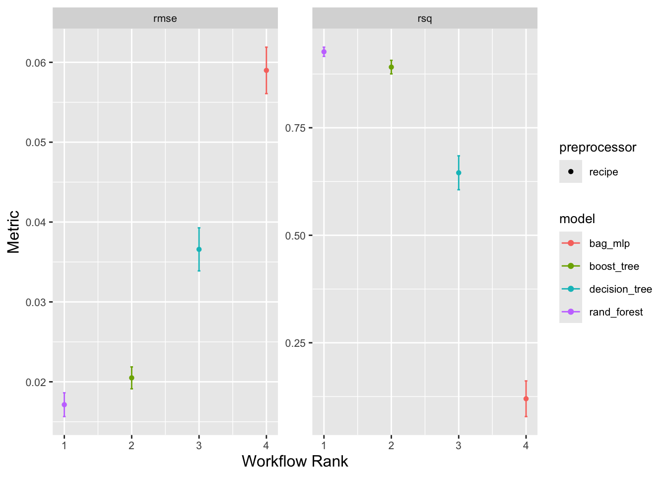
Figure 7. Ranking different models’ root mean squared error and R-squared error values, tested against CO2 per kilowatt hour emissions data for the top five cumulative CO2 emitters.

Table 4. Ranking Model Testing Results

In [30]:

rank_results(wf, rank_metric = "rsq", select_best = TRUE)

# A tibble: 8 × 9
  wflow_id         .config .metric   mean std_err     n preprocessor model  rank
  <chr>            <chr>   <chr>    <dbl>   <dbl> <int> <chr>        <chr> <int>
1 recipe_rand_for… Prepro… rmse    0.0171 9.04e-4    10 recipe       rand…     1
2 recipe_rand_for… Prepro… rsq     0.927  6.51e-3    10 recipe       rand…     1
3 recipe_boost_tr… Prepro… rmse    0.0205 8.33e-4    10 recipe       boos…     2
4 recipe_boost_tr… Prepro… rsq     0.891  9.56e-3    10 recipe       boos…     2
5 recipe_decision… Prepro… rmse    0.0366 1.64e-3    10 recipe       deci…     3
6 recipe_decision… Prepro… rsq     0.645  2.40e-2    10 recipe       deci…     3
7 recipe_bag_mlp   Prepro… rmse    0.0590 1.77e-3    10 recipe       bag_…     4
8 recipe_bag_mlp   Prepro… rsq     0.120  2.52e-2    10 recipe       bag_…     4

In [31]:

## Making a workflow to predict CO2 emitted per kilowatt-hour

library(tidymodels)
rf_wf <- workflow() %>%
  # Add the recipe
  add_recipe(rec_energy) %>%
  # Add the model
  add_model(rf) %>%
  # Fit the model to the training data
  fit(data = ghg_per_eny_train) 

rf_data <- augment(rf_wf, new_data = ghg_per_eny_test)

dim(rf_data)

[1] 158   9

In [32]:

# finding the most important predictors

rf_model <- extract_fit_engine(rf_wf)
vip::vip(rf_model) + theme(
    text = element_text(size = 12),
    axis.title = element_text(size = 14),
    axis.text = element_text(size = 10),
    plot.title = element_text(size = 16, face = "bold"),
    legend.title = element_text(size = 14),
    legend.text = element_text(size = 12))

ggsave(filename = "compare_pkwh.png", plot = last_plot(), path = "imgs" )

Saving 7 x 5 in image

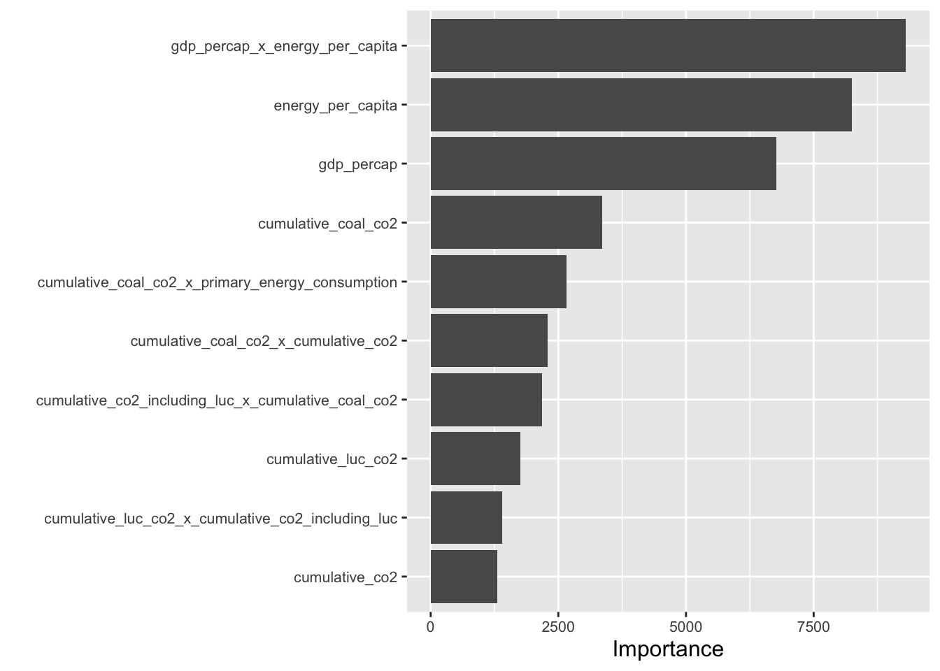
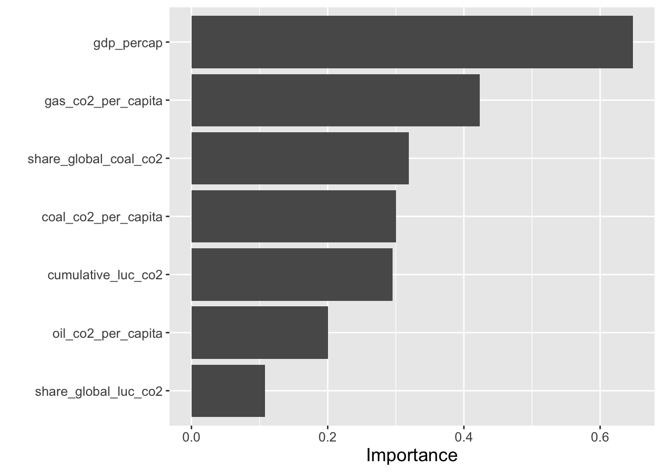
Figure 8. Ranking importance of each predictor variable at explaining CO2 emissions per kilowatt-hour in the random forest model selected for analysis.

Out of the four models tested to predict greenhouse gas emissions per capita (excluding land use change), a random forest model with ranger engine and regression mode was the most accurate. The second best was a boosted tree model. The 2 models had r-squared values of 0.92 and .89, respectively with RMSE = .01 and .020, respectively (Figure 1, Table 2). The most important predictor variables for greenhouse gas emissions per capita were (1) an interaction variable of gdp per capita and energy use per capita, (2) energy use per capita, and (3) gdp per capita (Figure 2). For predicting CO2 per kilowatt-hour, the random forest model with ranger engine and regression mode was the most accurate, with the second best also being a boosted tree model: The models also had and r-squared of 0.92 and .89, respectively with RMSE = .017 and .020 (Figure 4, Table 4). The top three predictor variables by importance for CO2 consumption per kilowatt hour were (1) gdp per capita, (2) CO2 emitted from gas consumption, and (3) CO2 emitted from oil consumption (Figure 5). ANOVA analysis of co2_per_unit_energy revealed that in terms of energy efficiency, Japan and Russia did not experience significant changes through COVID, while the other three countries did.

Analysis

In [33]:

## Making a correlation plot

library(corrplot)

corrplot 0.95 loaded

corrplot(pc_cor,
         method = "color",        # Color gradient
         type = "upper",          # Show upper triangle only
         diag = FALSE,            # Hide diagonal (1's)
         tl.col = "black",        # Text label color
         tl.srt = 45,             # Rotate variable names
         addCoef.col = "white",   # Add correlation coefficients
         number.cex = 0.7,        # Coefficient font size
         col = colorRampPalette(c("blue", "white", "red"))(100))

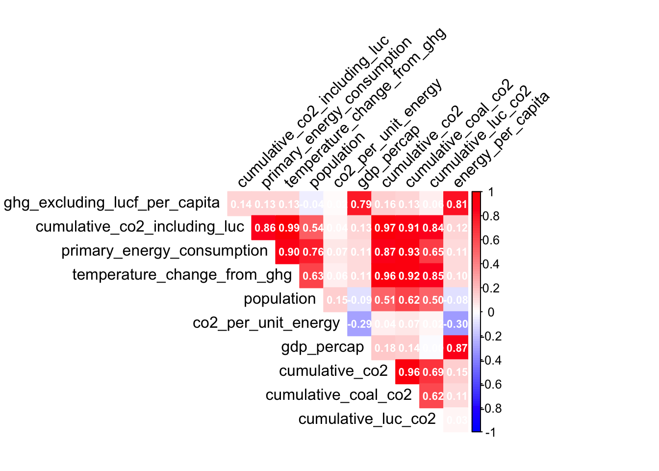
Figure 9. correlation table between predictor variables of GHG releaseed per capita excluding land use change per capita.

In [34]:

library(corrplot)

corrplot(pkwh_cor,
         method = "color",        # Color gradient
         type = "upper",          # Show upper triangle only
         diag = FALSE,            # Hide diagonal (1's)
         tl.col = "black",        # Text label color
         tl.srt = 45,             # Rotate variable names
         addCoef.col = "white",   # Add correlation coefficients
         number.cex = 0.7,        # Coefficient font size
         col = colorRampPalette(c("blue", "white", "red"))(100))

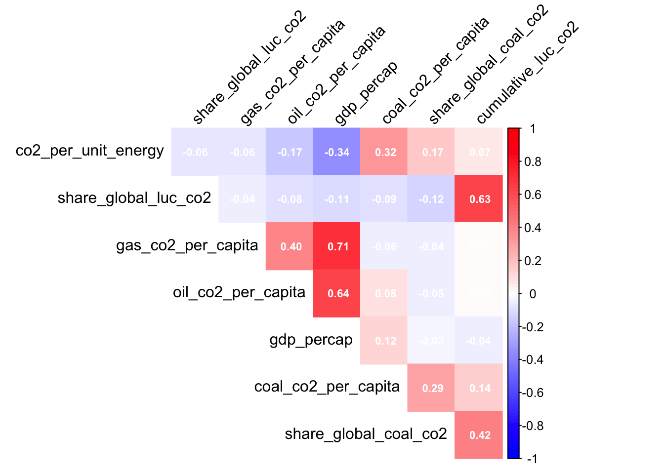
Figure 10. Correlation table between the variables predicting CO2 per unit energy. None of the variables had strong enough correlations to make interaction terms.

Included in CO2 per capita and CO2 per kilowatt-hour generated models, GDP per capita was a highly effective predictor variable because it was the third most important variable for greenhouse gas generation per capita and the most important variable for CO2 emissions per unit of energy generated. (figures 2 and 5). Mirziyoyeva and Salahodjaev (2023) confirm this trend with their own data. They also concluded that this relationship is inverse U-shaped, suggesting there are high emissions pressures at early stages of economic development that then slow down. There are emissions associated with every step of a product’s lifetime. In order from highest to lowest percent of total, energy (34%), industry (24%), agriculture, forestry, and other land use (22%) and shipping as well as both public and private transportation (15%) are involved. Higher associated activity explains correlations in figures 2 and 5. For CO2 emitted per kilowatt-hour, gas CO2 per capita was a close second behind GDP per capita (Figure 5). Natural gas is more favorable to coal because of its lower emissions. For example, the United States saw an 89 Mt increase in gas emissions in 2022 (International Energy Agency, 2022). Based on Figure 7, fewer variables were correlated when predicting CO2 per unit energy, suggesting a greater variety of predictors was responsible. In Figure 5, predictor variables are far closer together in importance than in Figure 2. Based on the predictor variables, this suggests causes of energy-related CO2 are more complex. Greenhouse gas emissions per capita were disproportionately affected by estimations of energy use and GDP, while other factors like coal CO2 were less than a third as important (Figure 5) Temperature change from greenhouse gas emissions was highly correlated with sector-specific emissions like coal as well as total CO2 emissions and even overall energy usage, so interaction terms were added to the model (Figure 6). However, the GHG variable importance model did not rank temperature change from emissions among the top ten predictor variables. Emissions are really a proxy for measuring each country’s global warming responsibility. Temperature change’s strong relationship with predictor variables but not with GHG per capita is expected because some countries can have high per capita emissions but small populations. Still, temperature’s correlations with primary energy consumption (0.90), cumulative CO2 including land use change (0.99), cumulative coal emissions (0.92), and cumulative land use change (.85) support these metrics as estimates of climate change. Primary energy consumption in particular is less directly related to greenhouse gases, but up until present energy consumption is related to global warming because of the interconnectivity of these predictors (Figure 10).

Discussion

Energy consumption can decouple with emissions-related warming with a greater adoption of renewable energy sources Mirziyoyeva & Salahodjaev (2023) . Energy-related CO2 emissions can be reduced by paying attention to factors like nighttime lights, which were correlated with higher overall emissions Xie et al. (2025). There are several reasons why GDP per capita is such an effective predictor of GHG emissions. Mirziyoyeva and Salahodjaev (2023) point out GDP’s consistent role in emissions.

One aspect of GDP and emissions that we did not examine was international trade’s role in carbon emissions. The import and export of products is harder to attribute to any one country, especially with overseas shipping on cargo carriers. These vessels emit large amounts of greenhouse gases and have been the subject of Our World In Data’s study as well. According to the International Energy Agency (2019), one-fifth of the world’s CO2 comes from global transport I. E. Agency (2023).

A step to take for future modeling would be to examine what aspects of GDP have the potential to emit fewer greenhouse gases. Currently, economic growth in several upper-income countries has decoupled from emissions per capita, even accounting for offshored production Ritchie (2021). Some countries demonstrate high GDP per capita but have lower emissions and can be a model for the rest of the world. Franco et al. (2023) note that economic factors are an indicator of emissions because of the energy costs of the economic system, especially in cities Franco et al. (2023).

The heavy influence of GDP on emissions highlights how important it is for wealthier countries to invest in decarbonization. The effect of gas and oil on per-capita emissions is likely due to transportation, as countries with a large number of personal vehicles require a significant amount of fuel (which leads to more emissions). Coal and land use are more reflective of broad systemic factors, and therefore would not have as significant of an effect on personal emissions. They are more reflective of how efficiently a country produces and uses energy.

The countries we looked at emit most of their CO2 from industry, but there are developing countries with high emissions from land use change—most notably Brazil Ritchie et al. (2023). Khajavi and Rastgoo (2020) also found that a hybrid random forest model was best at predicting CO2 emissions from road transport@khajavi_rastgoo_2023. Due to the COVID lockdown, transportation emissions would have decreased significantly as travel was banned or highly discouraged. Deweese et al. (2022) state that travel-based emissions fell by 36% in April of 2020 DeWeese et al. (2022). Although travel is one of the largest contributors to greenhouse gas emissions, accounting for all emissions from both public and private sectors is complicated, particularly for tourism Qin et al. (2023).

Conclusions

According to our analysis, we found that on average, emissions fell considerably during the peak of the COVID-19 pandemic, before rebounding in the following year. This was particularly apparent in oil and gas usage, which falls in line with the decreased usage of transportation during lockdowns. Along with these general trends, there were more specific changes relating to each of the five top emitters. According to ANOVA analysis, China, India, and the US showed significant changes in emission levels per unit energy, while Japan and Russia did not change in statistically significant ways. This tells us that the energy efficiency of these two countries has more of a capacity to remain stable during shocks. Coal and land use were heavy predictors of energy efficiency, as these two factors are tied to how efficiently a country’s infrastructure handles energy production and dispersion. ANOVA analysis also concluded that China, Japan, and the US had statistically significant changes in per capita emissions, while India and Russia did not. From this, we can conclude that for these two countries, per-person sources of emissions remained constant throughout the pandemic. Oil and gas usage were signifcant indicators of per capita emissions, which aligns with the nature of oil and gas-powered transportation.

By predicting both greenhouse gas emissions per capita and CO2 from energy use before, during, and after the COVID-19 era, we used two distinct and relatable lenses to view the climate crisis. Up until the present, CO2 emissions related to energy and CO2 emissions per capita were closely tied to GDP per capita.

Gas consumption and coal consumption account for the greatest energy use after GDP, with gas reflecting trends toward this lower-emissions form of energy production. Coal has a high rate of CO2 emissions, which places it third in predicting CO2 emissions per unit energy. Energy use accounts for the most GHG emissions per capita.

Current trends in preferred energy sources reflect energy-related emissions, while emissions per capita reflect overall performance. As the renewable energy transition accelerates in countries with developing GDPs, we will continue preparing for a gap between economic growth and emissions.

Agency, E. P. (2025). Sources of greenhouse gas emissions. In United States Environmental Protection Agency. https://www.epa.gov/ghgemissions/sources-greenhouse-gas-emissions

Agency, I. E. (2023). CO2 emissions in 2022. In IEA. IEA. https://www.iea.org/reports/co2-emissions-in-2022

Archer, D., Eby, M., Brovkin, V., Ridgwell, A., Cao, L., Mikolajewicz, U., Caldeira, K., Matsumoto, K., Munhoven, G., Montenegro, A., et al. (2009). Atmospheric lifetime of fossil fuel carbon dioxide. Annual Review of Earth and Planetary Sciences, 37, 117–134. https://doi.org/10.1146/annurev.earth.031208.100206

DeWeese, J., Ravensbergen, L., & El-Geneidy, A. (2022). Travel behaviour and greenhouse gas emissions during the COVID-19 pandemic: A case study in a university setting. Transportation Research Interdisciplinary Perspectives, 12, 100531. https://doi.org/10.1016/j.trip.2021.100531

Franco, C., Melica, G., Treville, A., Baldi, M. G., Ortega, A., Bertoldi, P., & Thiel, C. (2023). Key predictors of greenhouse gas emissions for cities committing to mitigate and adapt to climate change. Cities, 137, 104342. https://doi.org/10.1016/j.cities.2023.104342

Giannelos, S., Bellizio, F., Strbac, G., & Zhang, T. (2024). Machine learning approaches for predictions of CO2 emissions in the building sector. Electric Power Systems Research, 235, 110735. https://doi.org/10.1016/j.epsr.2024.110735

Mirziyoyeva, Z., & Salahodjaev, R. (2023). Renewable energy, GDP and CO2 emissions in high-globalized countries. Frontiers in Energy Research, 11. https://doi.org/10.3389/fenrg.2023.1123269

Programme, U. N. E. (2022). Emissions gap report 2022: The closing window.

Qin, F., Liu, J., & Li, G. (2023). Accounting for tourism carbon emissions: A consumption stripping perspective based on the tourism satellite account. Tourism Economics, 30(3), 633–654. https://doi.org/10.1177/13548166231175378

Rahman, M. M., Shafiullah, M., Alam, M. S., Rahman, M. S., Alsanad, M. A., Islam, M. M., Islam, M. K., & Rahman, S. M. (2023). Decision tree-based ensemble model for predicting national greenhouse gas emissions in saudi arabia. Applied Sciences, 13(6), 3832. https://doi.org/10.3390/app13063832

Ritchie, H. (2021). Many countries have decoupled economic growth from CO2 emissions, even if we take offshored production into account. In Our World in Data. https://ourworldindata.org/co2-gdp-decoupling

Ritchie, H., Rosado, P., & Roser, M. (2023). CO2 and greenhouse gas emissions. Our World in Data. https://ourworldindata.org/co2-and-greenhouse-gas-emissions

Samborska, V. (2025). Scaling up: How increasing inputs has made artificial intelligence more capable. Our World in Data.

Si, M., & Du, K. (2020). Development of a predictive emissions model using a gradient boosting machine learning method. Environmental Technology & Innovation, 20, 101028. https://doi.org/10.1016/j.eti.2020.101028

Xie, Y., Liu, R., & Fan, M. (2025). Spatial and temporal variation in energy-based carbon dioxide emissions and their predictions at city scale in future, china. Process Safety and Environmental Protection, 193, 1–25. https://doi.org/10.1016/j.psep.2024.11.032